Basic Usage#
This section will help you get started with prolint2, from loading the trajectory to basic analyses of the interactions. It is recommended to use prolint2 within a Jupyter notebook environment for a more interactive and convenient experience. Here are the essential steps to complete the most basic workflow:
Import the prolint2 Universe:
In your Python environment, import the ProLint2 Universe class as:
from prolint2 import Universe
This class allows you to load your simulation data and get basic topological information of your system.
Load Your Data
Use the ProLint2 Universe class to load your simulation data, typically a GRO file for coordinates and an XTC file for trajectory. In this case, it will be used a sample data included in the library for a G protein-coupled inwardly rectifying potassium channel (GIRK).
Importing the GIRK sample data:
from prolint2.sampledata import GIRKDataSample
GIRK = GIRKDataSample()
You can then load the trajectory data:
u = Universe(GIRK.coordinates, GIRK.trajectory)
Now, you have a Universe object u that you can use for further analysis.
Understand Query and Database
prolint2 uses the concepts of query and database groups for defining the interactions. See previous section (Workflow) for more information on this.
You can access these groups using the query and database attributes. For example, we can access the number of atoms in each group as follows:
n_query_atoms = u.query.n_atoms
n_database_atoms = u.database.n_atoms

print(f'Number of query atoms: {n_query_atoms}')
print(f'Number of database atoms: {n_database_atoms}')
This setup allows you to analyze interactions between the query and the database by initializing a Contacts object.
Compute Contacts
To compute contacts between the query and database groups, you can use the compute_contacts method. This method requires a cutoff distance in Angstroms for defining contacts:
contacts = u.compute_contacts(cutoff=7)
This step might take a few seconds, as it is calculating the interactions in every frame of the trajectory.
Define Metrics
Computing contact metrics is straightforward. You can create instances of various metrics, such as MeanMetric, and apply them to your contacts:
from prolint2.metrics.metrics import Metric, MeanMetric

mean_instance = MeanMetric() # create an instance of the MeanMetric class
metric_instance = Metric(contacts, mean_instance) # feed the contacts and the above instance to the Metric class
mean_contacts = metric_instance.compute() # compute the metric
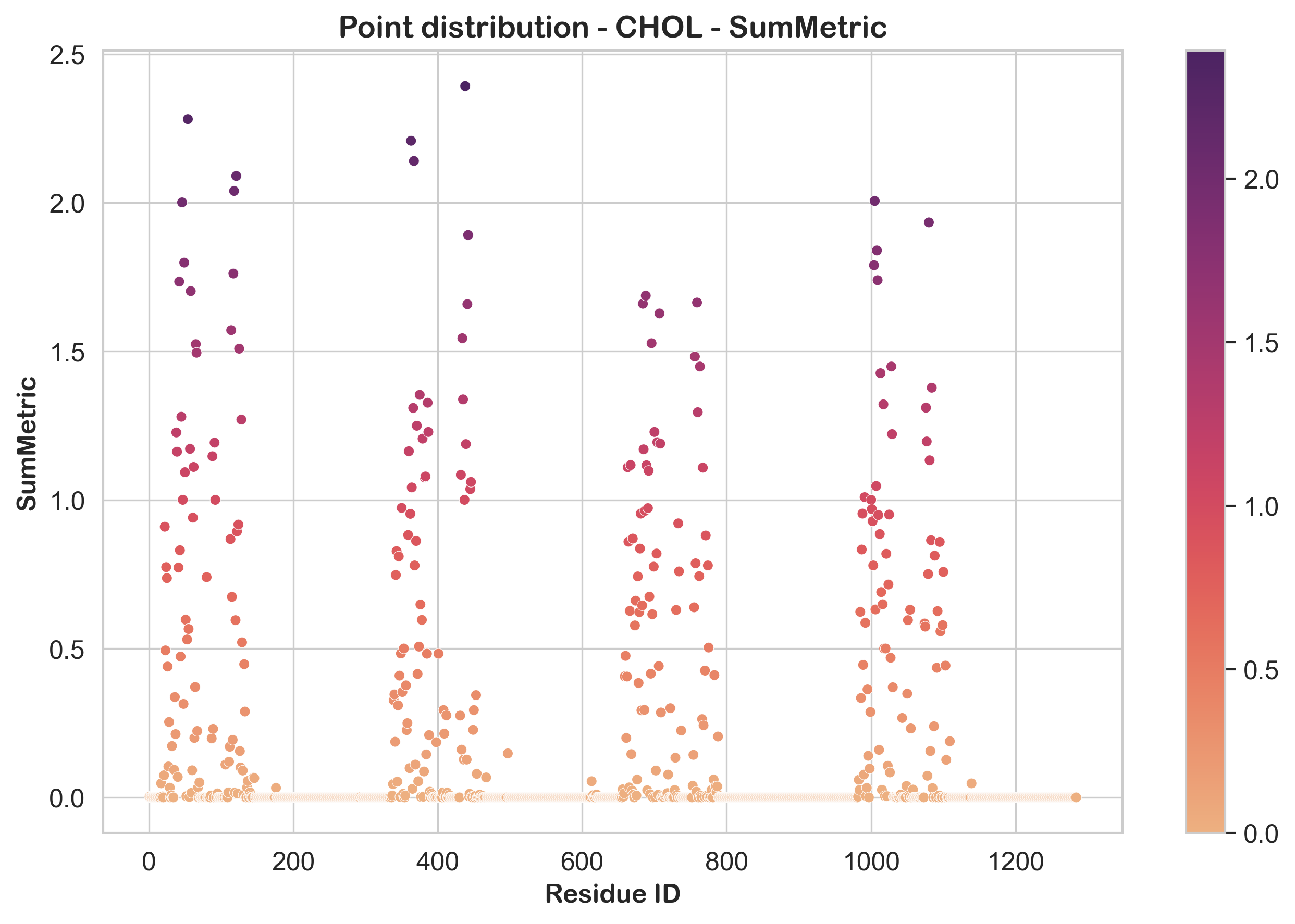
Using Plotters to visualize interactions
To visualize the interactions, you can use prolint2’s Plotters. Here is an example of how to create a Point Distribution plot:
from prolint2.plotting import PointDistribution

PD = PointDistribution(u, mean_contacts, fig_size=(8, 5))
PD.create_plot(lipid_type='CHOL', metric_name='MeanMetric', linewidth=0.24, palette='flare')