ProLint Workflow¶

This tutorial covers a complete ProLint workflow: loading simulation data, computing contacts, running analyses, and generating visualizations.

Step 1: Load Your Simulation¶

ProLint extends the MDAnalysis Universe with additional properties and methods for biomolecular interaction analysis. Start by creating a ProLint Universe as follows:

from prolint import Universe, setup_logging
import logging

# Enable logging to see progress
setup_logging(level=logging.INFO)

# Load your simulation files
universe = Universe("topology.gro", "trajectory.xtc")

# Check what was loaded
print(f"Trajectory: {universe.trajectory.n_frames} frames")
print(f"Query atoms: {universe.query.n_atoms} (protein)")
print(f"Database atoms: {universe.database.n_atoms} (non-protein)")

Custom Selections¶

By default, ProLint automatically identifies:

Query: All protein atoms
Database: All non-protein atoms (lipids, ligands, water, ions)

The query and database properties are extended MDAnalysis AtomGroup objects defining the two groups for contact analysis. The query is the molecule of interest (e.g., a protein) whose residues you want to characterize. The database contains the interaction partners (e.g., lipids, ligands) that may contact the query. ProLint allows to customize both using standard MDAnalysis selection syntax:

# Focus on specific residues
universe.query = universe.select_atoms("protein and resid 1-100")

# Analyze only specific lipids in a membrane model
universe.database = universe.select_atoms("resname POPE CHOL")

# Check number of residues in query group
print(f"Number of query residues: {universe.query.residues.n_residues}")

# Check available molecule types in the database
print(f"Molecule types: {universe.database.unique_resnames}")
print(f"Database counts: {universe.database.resname_counts}")

Units and Normalization¶

The universe.params property shows the normalization method and time units used for results. By default, normalization is by contact counts (unitless). You can set normalization to actual_time to report results in physical time units:

# Default params
print(f'Default parameters for contact calculations: {universe.params}')

# Change normalization method to 'actual time'
universe.normalize_by = 'actual_time'
universe.units = 'ns'

# Modified params
print(f"Modified parameters: {universe.params}")

Step 2: Compute Contacts¶

Compute distance-based contacts between query and database groups:

# Compute contacts with 7 Angstrom cutoff
contacts = universe.compute_contacts(cutoff=7.0)

For large trajectories, analyze a subset of frames:

contacts = universe.compute_contacts(cutoff=7.0, step=10)

Note

Working with Multi-Replica Systems

If your simulation contains multiple copies of the query (i.e.: protein replicas), ProLint can detect and handle them automatically. When fragments share the same residue IDs, they will be identified as replicas and you must specify which one to analyze using the replica parameter:

from prolint.core.replica_detection import detect_replicas

# Check for replicas in your system
result = detect_replicas(universe.query)
print(f"Found {result.n_replicas} replicas")
for info in result.replica_info:
    print(f"  Replica {info.replica_id}: {info.n_residues} residues")

# Analyze a specific replica
contacts = universe.compute_contacts(cutoff=7.0, replica='A')

To analyze all replicas together (useful for molecular complexes), ensure each has unique residue IDs with no overlap. ProLint will then process them collectively without requiring the replica parameter.

The contacts object stores all detected contacts and provides methods for analysis.

Step 3: Explore Contacts and Run Analyses¶

Explore the raw contact data before running analyses:

# Access frame-level contact data
# Structure: {query_resid: {database_resid: [frame_indices]}}
contact_frames = contacts.contact_frames

# See which lipids contact residue 42
if 42 in contact_frames:
    for lipid_id, frames in contact_frames[42].items():
        print(f"Residue 42 contacts lipid {lipid_id} in {len(frames)} frames")

# Access aggregated durations
# Structure: {query_resid: {lipid_type: {database_resid: [durations]}}}
contact_durations = contacts.contacts

# Quick metric computation
occupancy = contacts.compute_metric("occupancy", target_resname="CHOL")
for resid in [42, 43, 46]:
    if resid in occupancy and 'CHOL' in occupancy[resid]:
        occ = occupancy[resid]['CHOL']['global']
        print(f"Residue {resid} CHOL occupancy: {occ:.1%}")

ProLint provides nine built-in analysis types, each returning a result object with a data property containing the output. Here we demonstrate the timeseries analysis; see the Analyses and Visualizations Tutorial for all available analyses.

Time Series¶

Track contact counts over time:

# Contact counts per frame for each residue
ts_result = contacts.analyze(
    "timeseries",
    database_type="CHOL"
)

# Access the data
print(f"Residues analyzed: {len(ts_result.data['query_residues'])}")
print(f"Frames analyzed: {len(ts_result.data['frames'])}")

Step 4: Create Visualizations¶

Use the plot() function to visualize results.

from prolint.plotting import plot, apply_prolint_style

# Apply consistent styling
apply_prolint_style()

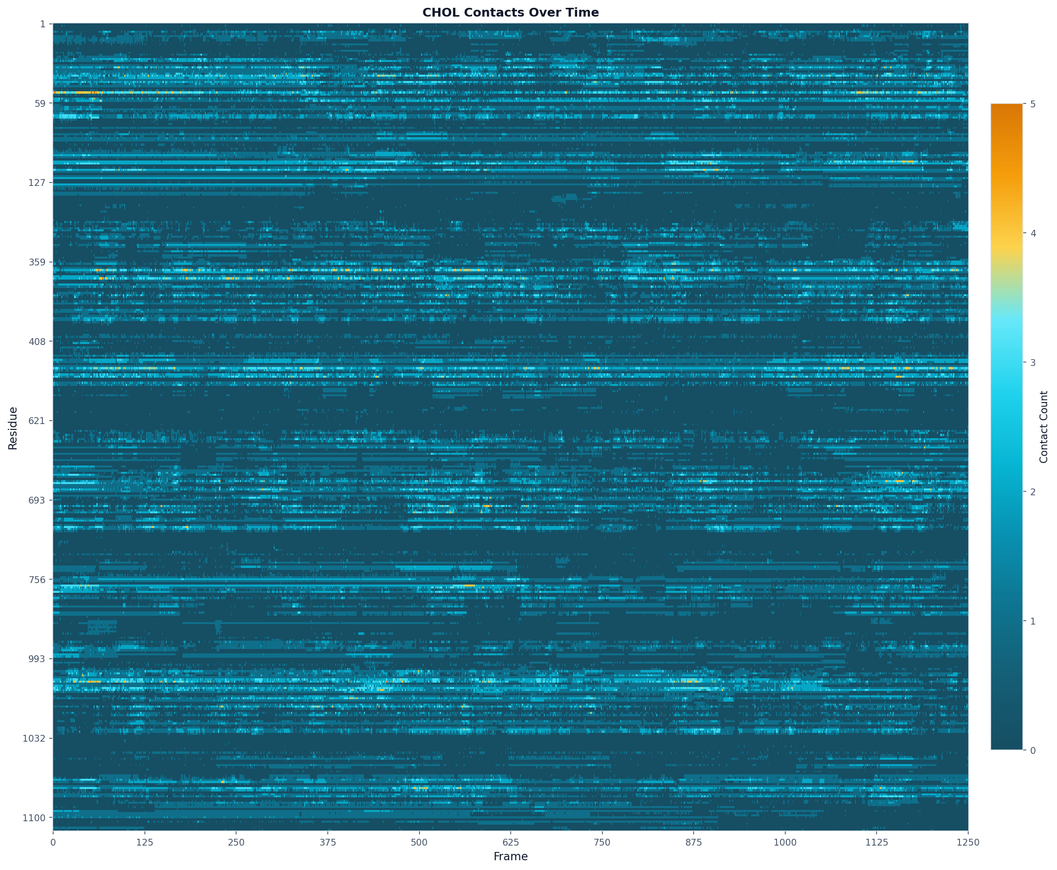
# Contact heatmap
fig, ax = plot(
    "heatmap",
    ts_result,
    colorscheme="prolint",
    max_display_cols=2000,
    title="CHOL Contacts Over Time"
)
fig.savefig("chol_contacts.png", dpi=150, bbox_inches="tight")

Complete Example Script¶

The following script combines all steps into a single workflow:

#!/usr/bin/env python
"""Basic ProLint workflow."""

import logging
from prolint import Universe, setup_logging
from prolint.plotting import plot, apply_prolint_style

# Setup
setup_logging(level=logging.INFO)
apply_prolint_style()

# Load simulation
universe = Universe("system.gro", "trajectory.xtc")
print(f"Loaded {universe.trajectory.n_frames} frames")
print(f"Database types: {universe.database.unique_resnames}")

# Compute contacts
contacts = universe.compute_contacts(cutoff=7.0)

# Run timeseries analysis
ts_result = contacts.analyze("timeseries", database_type="CHOL")

# Visualize
fig, ax = plot("heatmap", ts_result, title="CHOL Contacts Over Time")
fig.savefig("chol_contacts.png", dpi=150)
print("Saved chol_contacts.png")