Web Dashboard
ProLint provides a web-based dashboard for interactive analysis. Access it at https://prolint.ca.
The dashboard has two main pages:
Compute Page: Upload files, configure parameters, and run computations
View Page: Explore results with interactive visualizations
Compute Page
The Compute page guides you through loading data and running contact computations.
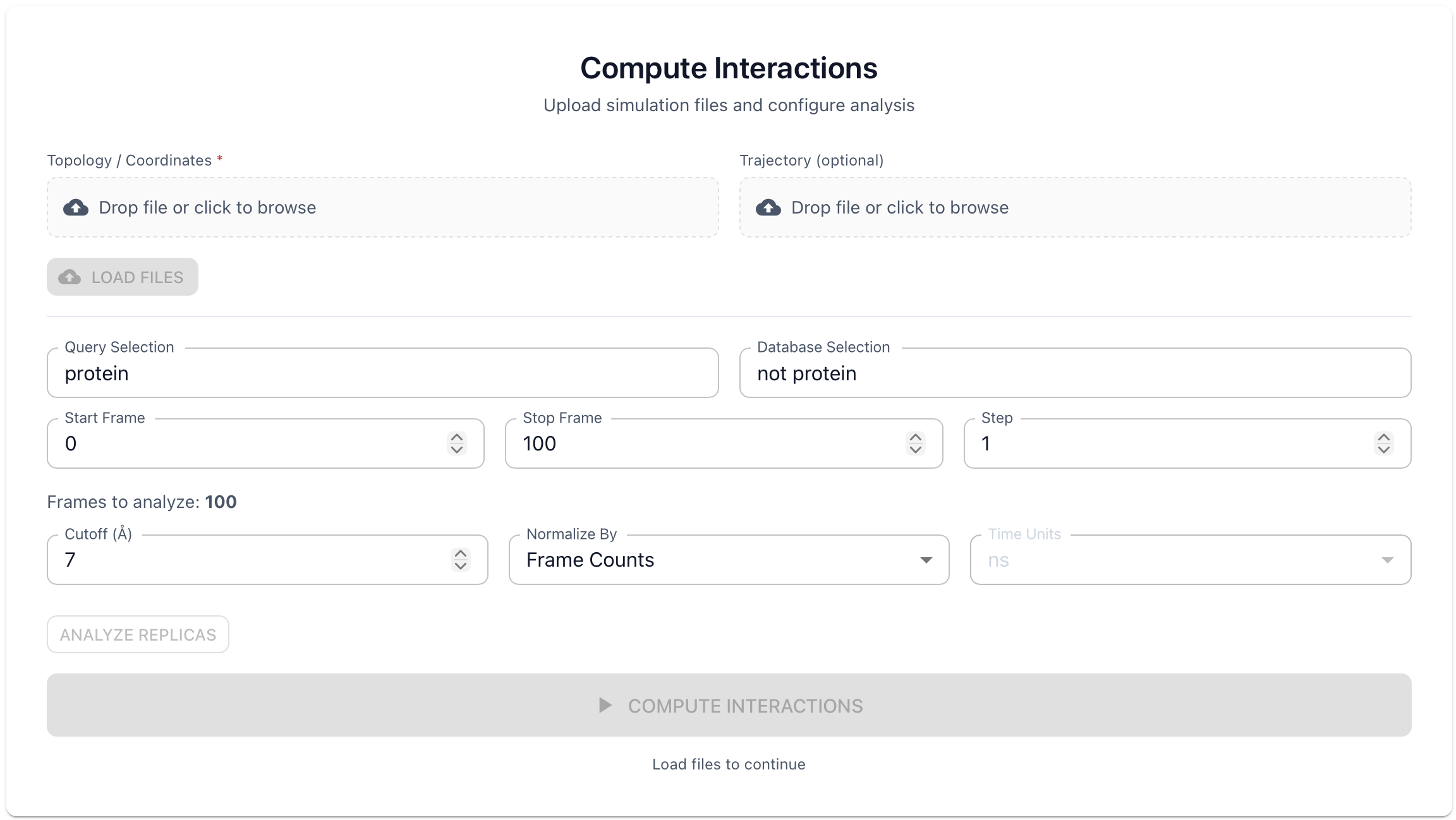
Upload Files
Topology File (required)
Drag and drop or click to upload your topology file. Supported formats include .gro, .pdb, .tpr, .psf, .mol2, and .xyz.
Trajectory File (optional)
For multi-frame analysis, also upload a trajectory: .xtc, .trr, .dcd, or .nc.
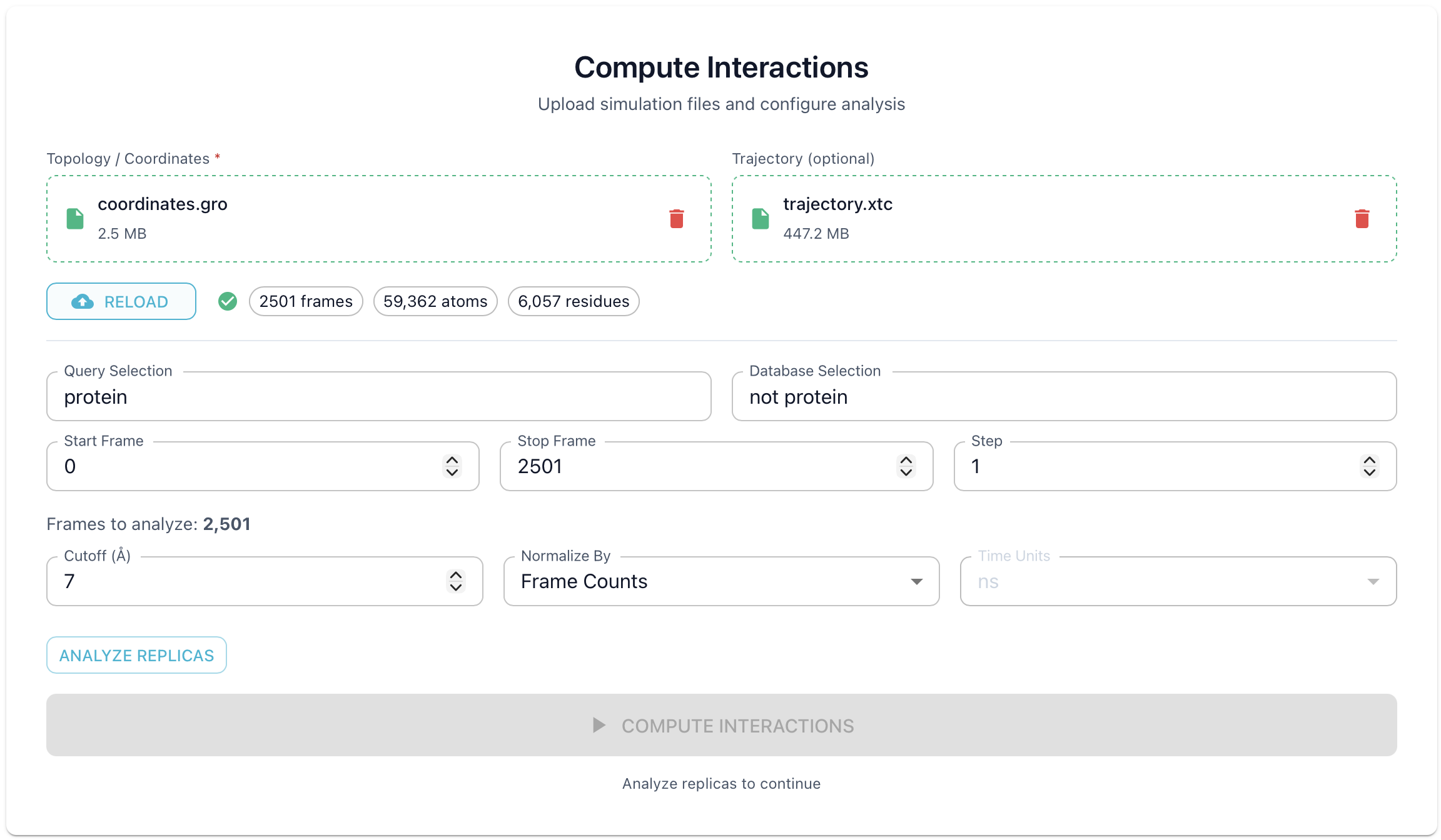
After upload, the dashboard displays dataset metadata including number of frames, atoms, and residues.
Configure Parameters
Atom Selections
Use MDAnalysis selection syntax to define what to analyze:
Query Selection: Atoms to analyze, set to
proteinby defaultDatabase Selection: Reference atoms for contacts, set to
not proteinby default
Selection examples:
protein— All protein atomsresname POPC POPE CHOL— Specific lipid typesresid 1-100— Specific residue range
Frame Range
Start Frame: First frame (0-indexed)
End Frame: Last frame (leave empty for all)
Step: Frame stride (1 = every frame, 10 = every 10th)
Tip
The dashboard allows a maximum of 5,000 frames per computation. For larger trajectories, adjust the step value to stay within this limit (e.g., for a 50,000 frame trajectory, use step ≥ 10). Start with a higher step to quickly preview results, then reduce it for finer analysis.
Distance Cutoff
Maximum distance (in Ångströms) for detecting contacts. Default is 7.0 Å.
Analyze Replicas
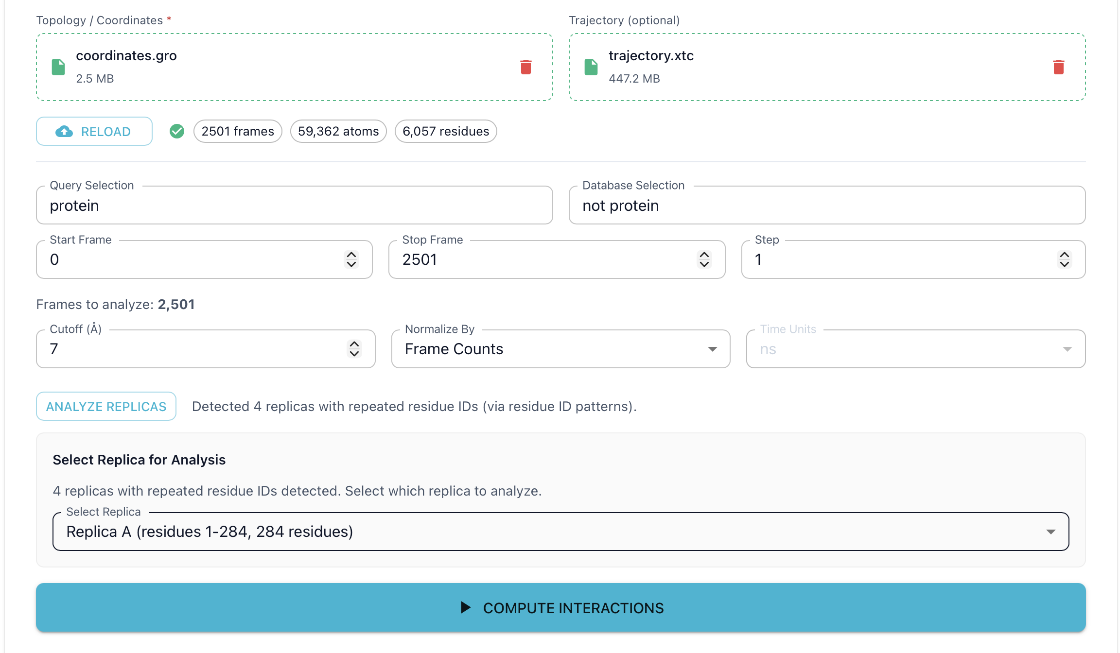
Before running the computation, click the “Analyze Replicas” button to check if your query selection contains multiple copies (replicas) of the same molecule. This step is required before computing contacts.
If replicas with overlapping residue IDs are detected, a dropdown will appear allowing you to select which replica to analyze
Select the desired replica from the dropdown (e.g., “Replica A”) to proceed
Note
To analyze all replicas together (e.g., for multimer complexes), ensure each replica has unique residue IDs with no overlap in your input files. ProLint will then process them collectively without requiring a replica selection.
Run Computation
Click “Compute Interactions” to start the analysis. A progress indicator shows computation status.
When complete, you’ll see a Result ID and computation time. Click “View Results” to navigate to the View page.
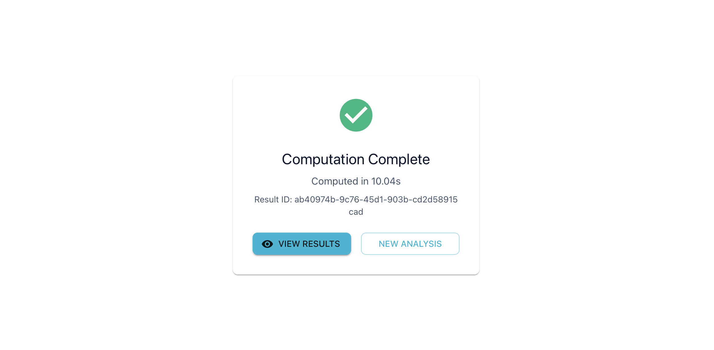
Note
Save your Result ID to return to your results later.
View Page
The View page provides interactive visualizations of your computed contacts.
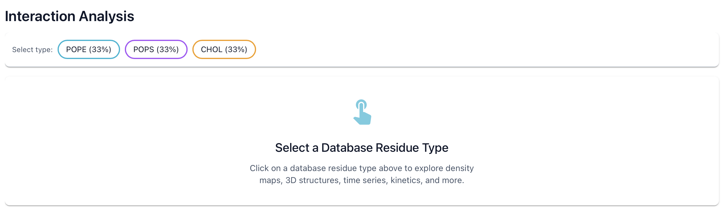
Database Type Filter
Use the individual buttons to filter results by molecule type. This updates all visualizations.
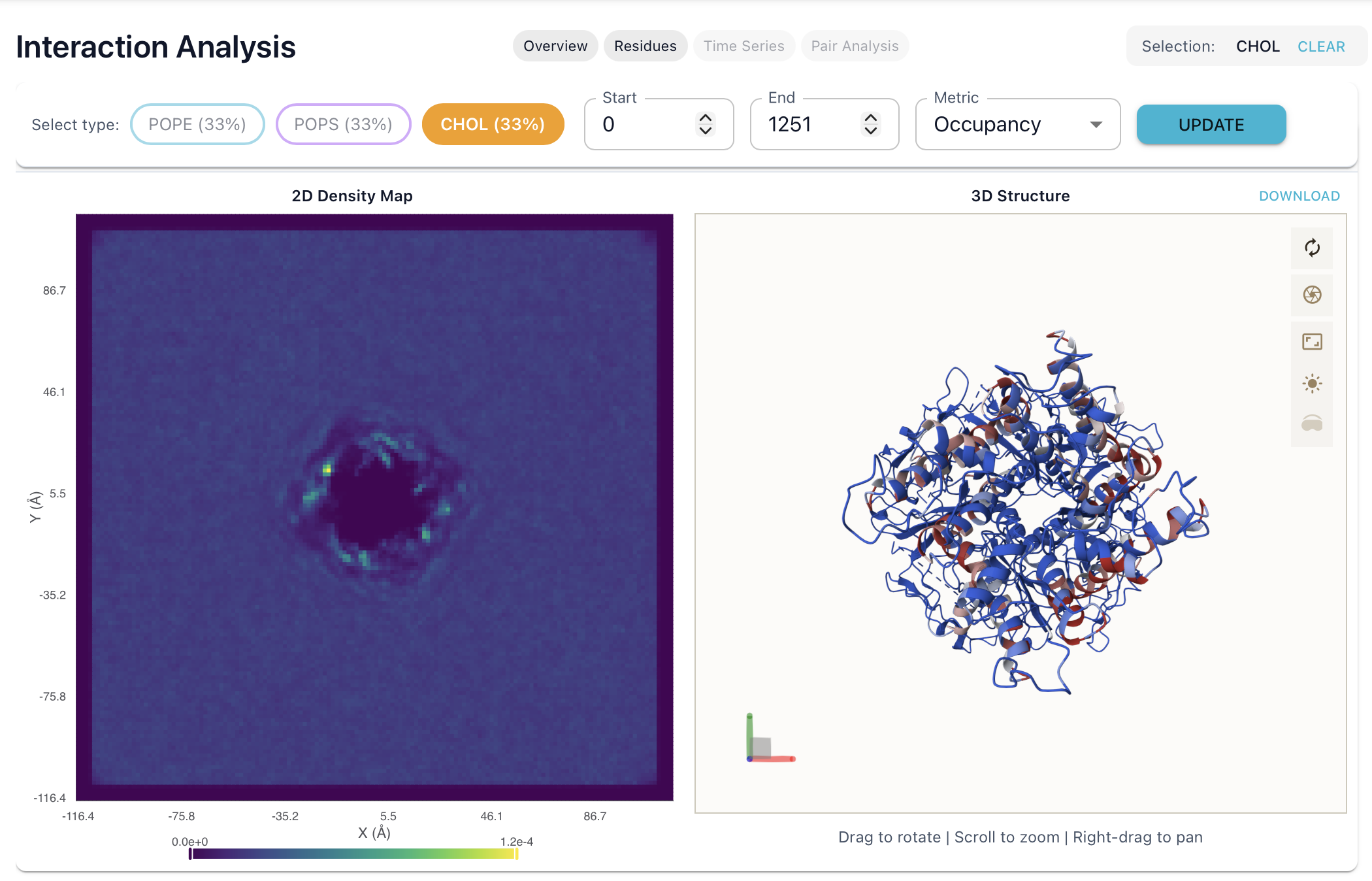
2D Density Map
Spatial distribution of database molecules around the query structure.
2D view showing where molecules preferentially locate
Color intensity indicates density (brighter = more frequent)
Use this to identify enrichment or depletion zones around specific regions of the query.
3D Projection Viewer
Interactive 3D visualization using Mol*.
Query structure colored by metric (occupancy, mean contacts, etc.)
Rotate, zoom, and pan with mouse controls
High and low contact regions highlighted
Controls: Left-click + drag to rotate, right-click + drag to pan, scroll to zoom.
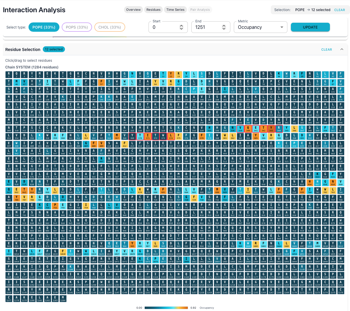
Metric Logo Plot
Sequence-level view of per-residue metrics across the query.
Each residue displayed as a single-letter code
Color intensity reflects metric value (occupancy, mean duration, etc.)
Hover over residues for detailed values
Click to select residues for further analysis
Use this to quickly identify hotspots along the sequence.
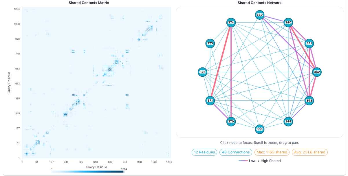
Shared Contacts Network
Network graph showing which residues contact the same database molecules.
Nodes represent query residues
Edges indicate shared contacts
Edge thickness reflects number of shared contacts
Draggable nodes with interactive layout
Use this to identify residue clusters that may form binding sites.
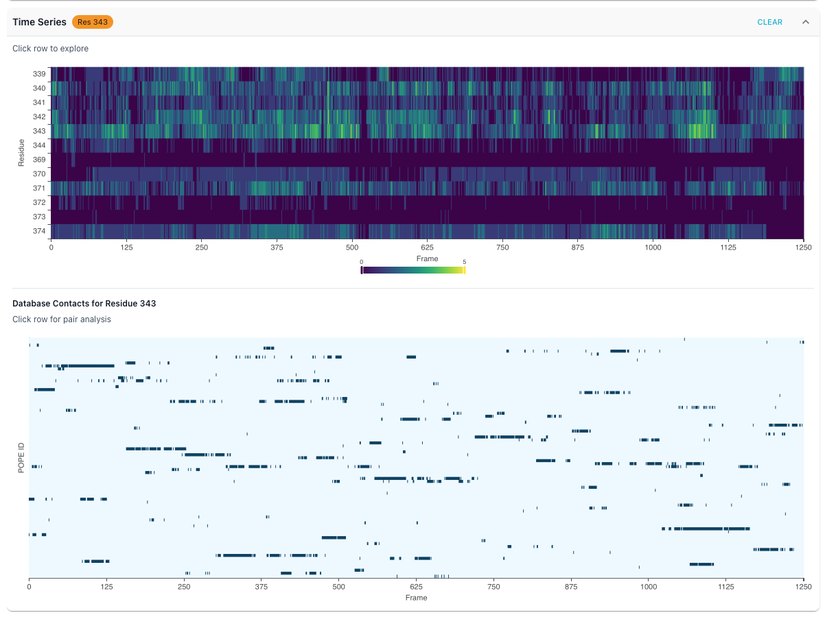
Time Series Plot
Line chart showing how contact counts change over the trajectory.
Select individual residues to compare
Frame-by-frame contact counts
Zoom and pan on time axis
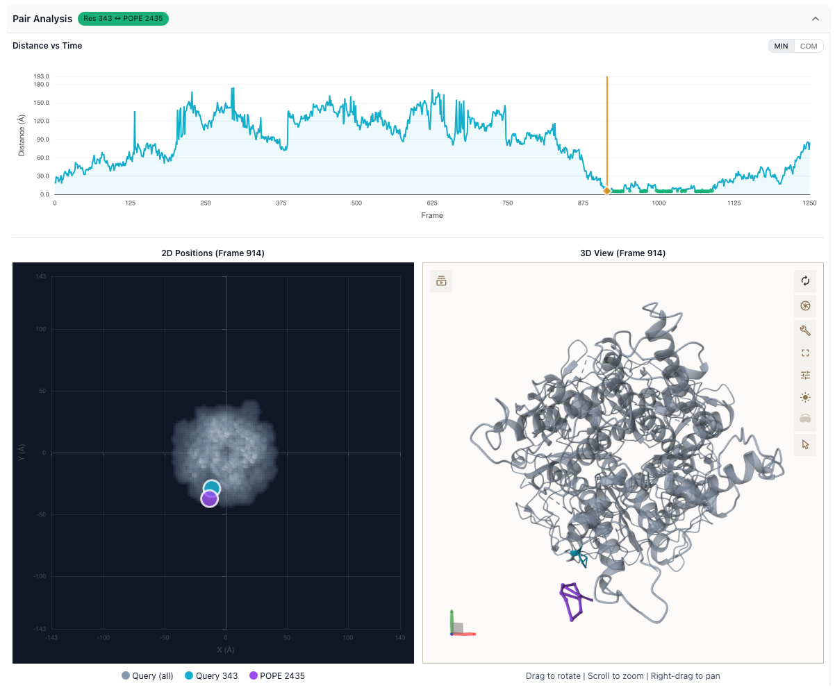
Distance Analysis
Track distances between specific query-database residue pairs over time.
Distance plotted frame-by-frame across the trajectory
Identify binding and unbinding events
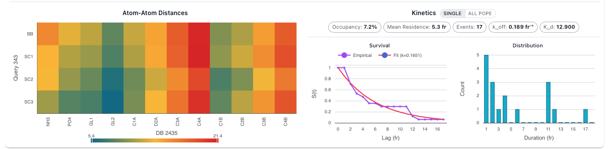
Kinetics Analysis
Detailed binding kinetics for selected residue-molecule pairs.
Survival Curve: Probability that a contact persists over time, with exponential fits
Residence Time Distribution: Histogram of contact durations
Kinetic Parameters: k_on, k_off, mean residence time, occupancy